Quantum Phase Estimation
Quantum phase estimation is a fundamental algorithm in quantum computing that allows us to estimate the phase of a quantum state associated with a QPU operation. In particular, it is used to determine the eigenvalues of a unitary operator. This is a crucial step in many quantum algorithms, including Shor’s algorithm for integer factorization and quantum simulation algorithms.
The basic idea of quantum phase estimation is to prepare a quantum state, apply the unitary operator whose eigenvalues we want to estimate, and then measure the state in a way that allows us to infer the phase of the eigenvalue. The algorithm uses a technique called the quantum Fourier transform, which is a quantum version of the classical discrete Fourier transform.
The quantum phase estimation algorithm consists of the following steps:
Preparation: Prepare two quantum registers. The first register contains a single qubit in the state |0⟩. The second register contains n qubits in the state |ψ⟩, which is the state whose eigenvalues we want to estimate.
Apply controlled unitary operations: Apply a series of controlled unitary operations to the second register with increasing powers of 2. The control qubits are the qubits in the first register, and the target qubits are the qubits in the second register. Specifically, if U is the unitary operator whose eigenvalues we want to estimate.
Apply inverse quantum Fourier transform: Apply the inverse quantum Fourier transform to the first register. This step allows us to convert the phase of the eigenvalue into a binary representation.
Measurement: Measure the first register on a computational basis. This gives us an estimate of the phase of the eigenvalue.
The output of the algorithm is a binary string representing the estimated phase of the eigenvalue. The probability of measuring a particular string is proportional to the squared modulus of the corresponding eigenvector coefficient.
Finally, quantum phase estimation is a powerful algorithm that allows us to estimate the phase of a quantum state and determine the eigenvalues of a unitary operator. It is a key component in many quantum algorithms and is an essential tool for quantum computing researchers.
#initialization
import matplotlib.pyplot as plt
import numpy as np
import math
from qiskit import IBMQ, Aer, transpile, assemble
from qiskit import QuantumCircuit, ClassicalRegister, QuantumRegister

from qiskit.visualization import plot_histogram

qpe = QuantumCircuit(4, 3)
qpe.x(3)
qpe.draw('mpl')

for qubit in range(3):
    qpe.h(qubit)
qpe.draw('mpl')


repetitions = 1
for counting_qubit in range(3):
    for i in range(repetitions):
        qpe.cp(math.pi/4, counting_qubit, 3); # This is CU
    repetitions *= 2


def qft_dagger(qc, n):
    """n-qubit QFTdagger the first n qubits in circ"""
    # Don't forget the Swaps!
    for qubit in range(n//2):
        qc.swap(qubit, n-qubit-1)
    for j in range(n):
        for m in range(j):
            qc.cp(-math.pi/float(2**(j-m)), m, j)
        qc.h(j)

qpe.barrier()
# Apply inverse QFT
qft_dagger(qpe, 3)
# Measure
qpe.barrier()
for n in range(3):
    qpe.measure(n,n)


aer_sim = Aer.get_backend('aer_simulator')
shots = 2048
t_qpe = transpile(qpe, aer_sim)
qobj = assemble(t_qpe, shots=shots)
results = aer_sim.run(qobj).result()
answer = results.get_counts()

plot_histogram(answer)


from fractions import Fraction
θ = 1/(2**3)
print(f'θ = {Fraction(θ)}')
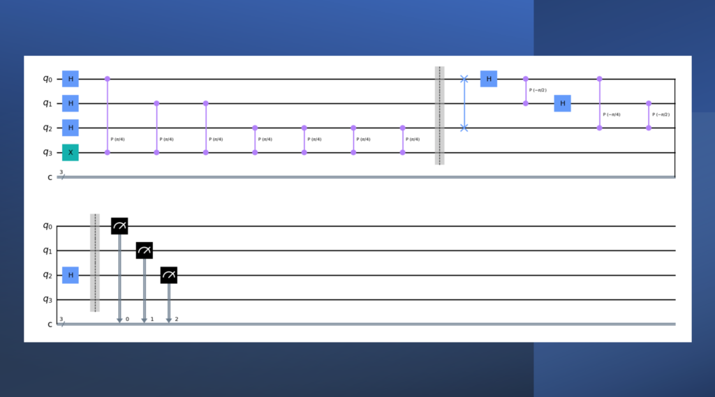
Below is the complete quantum circuit that we assembled for our Quantum Phase Estimation demo:

Here is the code snippet to demonstrate the implementation of QPE using Qiskit SKD. This code implements the Quantum Phase Estimation (QPE) algorithm using Qiskit, a quantum computing SDK. Here’s a step-by-step breakdown of the code:
- First, the necessary modules are imported: matplotlib.pyplot, numpy, math, IBMQ, Aer, transpile, assemble, QuantumCircuit, ClassicalRegister, QuantumRegister, and plot_histogram.
- Next, a QuantumCircuit object qpe with 4 quantum and 3 classical registers is created.
- The 4th qubit is initialized to the state |1> by applying an X gate.
- A Hadamard gate is applied to each of the first 3 qubits to create a superposition state.
- The cp gate (controlled phase shift) is applied to each qubit in the first 3 qubits, with the 4th qubit as the control and the angle of the phase shift doubling at each iteration. This creates a quantum circuit that performs the QPE algorithm.
- The qft_dagger function is defined, which implements the inverse Quantum Fourier Transform (QFT) on the first n qubits of a given quantum circuit. The QFT is an important part of the QPE algorithm.
- A barrier is applied to the quantum circuit to separate the QFT from the rest of the circuit.
- The inverse QFT is applied to the first 3 qubits using the qft_dagger function.
- The first 3 qubits are then measured, and the measurement results are stored in the first 3 classical registers.
- The aer_sim backend is set to the Aer simulator.
- The quantum circuit qpe is transpiled to the aer_sim backend and then assembled into a qobj with 2048 shots.
- The qobj is run on the aer_sim backend, and the results are stored in results.
- The counts of the measurement results are extracted from the results and stored in the answer.
- The measurement results are plotted as a histogram using plot_histogram.
In the last line, the code computes the value of θ = 1/(23) and prints it as a fraction using the Fraction class from the fractions module. This value represents the phase shift that was applied to the qubits during the QPE algorithm.

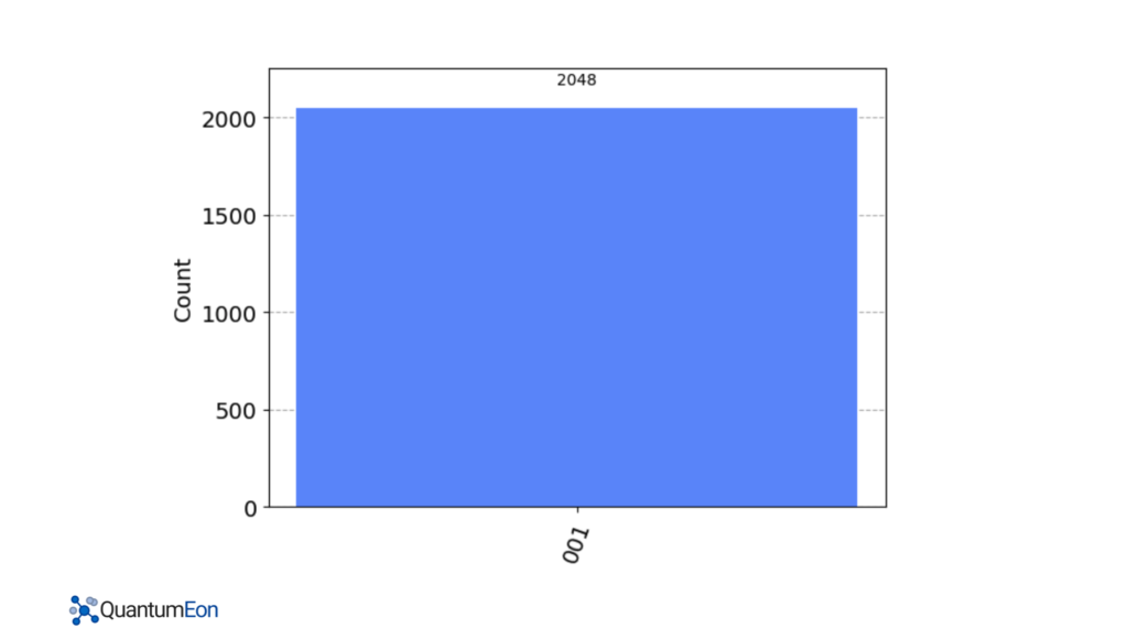
Which is exactly what we should expect. The QPE value is given by dividing The output of 001 = 1 by 8.
