
Quantum Neural Network
A quantum neural network (QNN) is a type of neural network that is implemented using quantum circuits. In a QNN, the basic building blocks of a classical neural network, such as neurons and synapses, are replaced with quantum counterparts that are implemented using quantum gates.
The basic working principle of a QNN is to encode classical data into quantum states, perform quantum operations on these states using quantum gates, and then extract the result in a classical form. This involves the use of quantum feature maps, which are used to encode the classical data into quantum states, and variational quantum circuits, which are used to manipulate these quantum states to perform the desired computations.
In a QNN, the parameters of the variational quantum circuits are optimized using classical optimization algorithms, such as gradient descent, to minimize a cost function that is defined based on the task at hand. This is done iteratively over multiple epochs until the cost function converges to a minimum value.
QNNs have the potential to provide significant speedups for certain tasks, such as pattern recognition and optimization, over classical neural networks. However, they also face significant challenges, such as noise and decoherence, that limit their practical implementation.
The code below implements a simple neural network using IBM Qiskit, a software framework for building and running quantum programs. This neural network aims to classify flowers from the iris dataset into two classes, using a quantum circuit to perform the classification.
The code starts by importing necessary libraries, including scikit-learn, Qiskit, NumPy, and Matplotlib. Then, it loads the iris dataset, selects the first 100 samples, and splits them into training and testing datasets.
Next, it defines a feature map function, which takes a sample from the dataset and maps it to a quantum circuit. The feature map uses N=4 quantum registers and applies a set of Rx gates to each register with values from the training set. Then, it defines a variational circuit function that applies controlled-not gates and Ry gates to the circuit, using random values of theta as parameters.
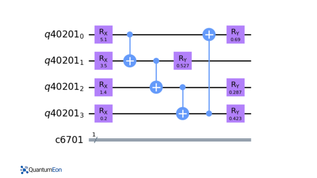
After that, it defines a quantum neural network function that uses the feature map and variational circuit functions to build a quantum circuit. It then measures the first register and executes the circuit on a quantum simulator backend to obtain the probability of measuring the “1” state. This probability is used as the prediction of the neural network for a given sample.
The code also defines a loss function, a gradient function, and an accuracy function. The loss function calculates the squared error between the prediction and the target value. The gradient function uses finite differences to estimate the gradient of the loss function with respect to the theta parameters. The accuracy function calculates the percentage of correctly classified samples in the training dataset.
The code trains the quantum neural network by performing a set number of epochs and updating the theta parameters using gradient descent with a fixed learning rate. It records the loss and accuracy at each epoch and plots the loss over time. It also compares the results of the quantum neural network with a classical support vector machine (SVM) classifier from scikit-learn on the testing dataset.
#Description: implementation of neural network using IBM qiskit

from sklearn import model_selection, datasets, svm
from qiskit import QuantumCircuit,Aer, IBMQ, QuantumRegister, ClassicalRegister
import qiskit
import numpy as np
import copy
import matplotlib.pyplot as plt

# Load dataset
iris = datasets.load_iris()
X = iris.data[0:100]
Y = iris.target[0:100]
X_train, X_test, Y_train, Y_test = model_selection.train_test_split(X,Y, test_size=0.33, random_state=40)

print(Y_train)

X_train

N = 4

def feature_map(X):
    q = QuantumRegister(N)
    c = ClassicalRegister(1)
    qc= QuantumCircuit(q,c)

    for i, x in enumerate(X_train[0]):
        qc.rx(x,i)

    return qc, c


qc , c = feature_map(X)

print(qc)


#Make the model more robust

def variational_circuit(qc, theta):

    for i in range(N-1):
        qc.cnot(i, i+1)
    qc.cnot(N-1, 0)
    for i in range(N):
        qc.ry(theta[i],i)
    return qc


qc = variational_circuit(qc, np.random.rand(N))


qc.draw('mpl')


#built neural network


def quantum_nn(X, theta, simulator = True):
    qc, c = feature_map(X)

    qc.barrier()
    qc = variational_circuit(qc, np.random.rand(N))
    qc.barrier()

    qc.measure(0,c)
    shots = 1E4
    backend = Aer.get_backend('qasm_simulator')
    job = qiskit.execute(qc,backend,shots =shots)
    result = job.result()
    counts = result.get_counts(qc)
    return counts['1']/shots


#Loss fucntion

def loss(prediction, target):
    return (target - prediction)**2


# ### Gradient function


def gradient(X,Y,theta):

    delta = 0.01
    grad = []
    for i in range(len(theta)):
        dtheta = copy.copy(theta)
        dtheta[i] += delta

        pred1 = quantum_nn(X, dtheta)
        pred2 = quantum_nn(X, theta)

        grad.append((loss(pred1, Y) - loss(pred2, Y))/delta)
        return np.array(grad)


#Accuracy

def accuracy(X, Y, theta):

    counter = 0
    for X_i, Y_i in zip(X, Y):
        prediction = quantum_nn(X_i, theta)

    if prediction < 0.5 and Y_i == 0:
        counter +=1
    elif prediction >= 0.5 and Y_i == 1:
        counter +=1

    return counter/len(Y)


#Train NN - Push data to the neural net
#learning rate
eta = 0.05
epoch = 25
loss_list = []

theta = np.ones(N)

print('Epoch \t Loss \t Training Accuracy')

for i in range(epoch):

    loss_tmp = []

    for X_i, Y_i in zip(X_train, Y_train):
        prediction = quantum_nn(X_i, theta)
        loss_tmp.append(loss(prediction, Y_i))
        theta = theta - eta * gradient(X_i, Y_i, theta)

    loss_list.append(np.mean(loss_tmp))
    acc = accuracy(X_train, Y_train, theta)

    print(f'{i} \t {loss_list[-1]:.3f} \t {acc:.3f}')


plt.plot(loss_list)
plt.xlabel('Epoch')
plt.ylabel('Loss')
plt.show()


qc.draw(output='mpl')

#Compare with classical ML

clf = svm.SVC()
clf.fit(X_train, Y_train)


print(clf.predict(X_test))
print(Y_test)
Again, this code provides a basic example of how to implement a quantum neural network using Qiskit and how to compare its performance with classical machine learning techniques. However, a more effective way to load data is missing here using the re-uploading data technique. I am going to elaborate on this technique in future posts.