Optimal Ground state of MOLECULES
Quantum computing has the potential to revolutionize the field of chemistry by enabling the simulation of molecular interactions and reactions with unprecedented accuracy and speed. This is because quantum mechanics is at the heart of chemistry, and quantum computers can leverage the inherent properties of quantum systems to solve problems that are intractable on classical computers.
One of the most promising applications of quantum computing in chemistry is in the calculation of molecular energies and structures. This is a key component of many chemical reactions and is typically carried out using computationally intensive methods like density functional theory (DFT) or Hartree-Fock theory. While these methods are powerful, they can be limited in their ability to predict the behavior of large, complex molecules accurately.
Quantum computers, on the other hand, can perform calculations using quantum algorithms that take advantage of the principles of superposition and entanglement to solve complex problems more efficiently. By simulating the behavior of molecules at the quantum level, quantum computers can provide more accurate predictions of molecular structures and energies, which can lead to a better understanding of chemical reactions and the design of new drugs and materials.
Another promising application of quantum computing in chemistry is in the simulation of chemical reactions. By simulating the quantum dynamics of a reaction, quantum computers can help to predict reaction rates and pathways, which can be used to optimize chemical processes or design new reaction pathways. This can greatly accelerate the development of new drugs, catalysts, and materials.
The ability of quantum computers to simulate quantum systems with unparalleled accuracy and speed has the potential to transform the field of chemistry by enabling new discoveries and breakthroughs in the design and optimization of chemical reactions and materials.
VQC stands for Variational Quantum Circuit, which is a type of quantum algorithm used to find the minimum energy state of a quantum system, such as a molecule.
In VQC, a quantum circuit is designed to prepare a trial wave function that is capable of representing the ground state of the system. This trial wave function is then used as input to a classical optimization algorithm, which adjusts the parameters of the quantum circuit to minimize the energy of the system. The process is repeated iteratively until the minimum energy state of the system is reached.
The reason why we need a variational quantum circuit to simulate the minimum ground state of molecules is because the problem of simulating the quantum behavior of molecules is extremely difficult for classical computers. This is because molecules are composed of many interacting quantum particles, such as electrons and nuclei, and the behavior of these particles is governed by the principles of quantum mechanics.
Variational quantum circuits, on the other hand, can exploit these particles’ quantum properties to simulate their behavior with greater efficiency than classical computers. By designing a quantum circuit that can prepare a trial wave function capable of representing the ground state of a molecule, we can use VQC algorithms to find the minimum energy state of the molecule with greater accuracy and speed than classical methods.
Broadly speaking, VQC algorithms represent a promising approach to solving the difficult problem of simulating the quantum behavior of molecules and may have important implications for the discovery and design of new materials and drugs.
Having obtained this information, it would be highly advantageous to develop a code that can efficiently determine the minimum ground state of an H3 molecule. This methodology can then be extended to other molecular structures with similar chemical properties.
This code below optimizes a molecular Hamiltonian’s ground state energy using the Ritz variational principle and the PennyLane library.
The molecular Hamiltonian is generated using the qchem module from PennyLane. The module uses the Hartree-Fock approximation to compute the molecular geometry and charge. The Hamiltonian is represented in the Jordan-Wigner representation.
The ansatz is defined using the double excitation gate, and the cost function is defined as the expectation value of the Hamiltonian. The Gradient Descent optimizer minimizes the cost function and finds the optimal circuit parameters that generate the ground state energy.
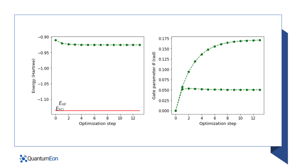
The code also computes the actual ground state energy of the Hamiltonian using the PennyLane library and plots the energy and gate parameters for each optimization step. The Full Configuration Interaction (FCI) energy computed classically is also plotted for comparison.
import pennylane as qml
from pennylane import numpy as np
from pennylane import qchem
import matplotlib.pyplot as plt


class QuantumChemistrySolver:
    def __init__(self, symbols, coordinates, charge=0):
        self.symbols = symbols
        self.coordinates = coordinates
        self.charge = charge

        self.hamiltonian, self.qubits = qchem.molecular_hamiltonian(
            self.symbols, self.coordinates, charge=self.charge
        )

        self.hf = qchem.hf_state(electrons=2, orbitals=6)

        self.num_wires = self.qubits
        self.dev = qml.device("lightning.qubit", wires=self.num_wires)

    def exp_energy(self, state):
        @qml.qnode(self.dev)
        def circuit(state):
            qml.BasisState(np.array(state), wires=range(self.num_wires))
            return qml.expval(self.hamiltonian)

        return circuit(state)

    def ansatz(self, params):
        @qml.qnode(self.dev)
        def circuit(hf, params):
            qml.BasisState(hf, wires=range(self.num_wires))
            qml.DoubleExcitation(params[0], wires=[0, 1, 2, 3])
            qml.DoubleExcitation(params[1], wires=[0, 1, 4, 5])

        return circuit(self.hf, params)

    def cost_function(self, params):
        return self.exp_energy(self.ansatz(params))

    def optimize(self, max_iterations=100, conv_tol=1e-06, stepsize=0.4):
        opt = qml.GradientDescentOptimizer(stepsize=stepsize)
        theta = np.array([0.0, 0.0], requires_grad=True)
        energy = [self.cost_function(theta)]
        angle = [theta]

        for n in range(max_iterations):
            theta, prev_energy = opt.step_and_cost(self.cost_function, theta)

            energy.append(self.cost_function(theta))
            angle.append(theta)

            conv = np.abs(energy[-1] - prev_energy)

            if n % 2 == 0:
                print(f"Step = {n},  Energy = {energy[-1]:.8f} Ha")

            if conv <= conv_tol:
                break

        print("\n" f"Final value of the ground-state energy = {energy[-1]:.4f} Ha")
        print("\n" f"Optimal value of the circuit parameter = {theta[0]:.4f} {theta[1]:.4f}")

        return theta, energy, angle

    def ground_state(self, params):
        @qml.qnode(self.dev)
        def circuit(hf, params):
            qml.BasisState(hf, wires=range(self.num_wires))
            qml.DoubleExcitation(params[0], wires=[0, 1, 2, 3])
            qml.DoubleExcitation(params[1], wires=[0, 1, 4, 5])
            return qml.state()

        return circuit(self.hf, params)

    def plot_energy_and_angles(self, energy, angle, E_fci, n):
        fig = plt.figure()
        fig.set_figheight(5)
        fig.set_figwidth(12)

        # Full configuration interaction (FCI) energy computed classically
        E_fci = -1.136189454088

        # Add energy plot on column 1
        ax1 = fig.add_subplot(121)
        ax1.plot(range(n + 2), energy, "go", ls="dashed")
        ax1.plot(range(n + 2), np.full(n + 2, E_fci), color="red")
        ax1.set_xlabel("Optimization step", fontsize=13)
        ax1.set_ylabel("Energy (Hartree)", fontsize=13)
        ax1.text(0.5, -1.1176, r"$E_\mathrm{HF}$", fontsize=15)
        ax1.text(0, -1.1357, r"$E_\mathrm{FCI}$", fontsize=15)
        plt.xticks(fontsize=12)
        plt.yticks(fontsize=12)

        # Add angle plot on column 2
        ax2 = fig.add_subplot(122)
        ax2.plot(range(n + 2), angle, "go", ls="dashed")
        ax2.set_xlabel("Optimization step", fontsize=13)
        ax2.set_ylabel("Gate parameter $\\theta$ (rad)", fontsize=13)
        plt.xticks(fontsize=12)
        plt.yticks(fontsize=12)

        plt.subplots_adjust(wspace=0.3, bottom=0.2)
        plt.show()
Upon executing the code, the resulting minimal ground state can be described as follows:
|ground_state> = 0.9960|110000> – 0.0852|001100> – 0.2508|000011>

