quanvolutional neural network
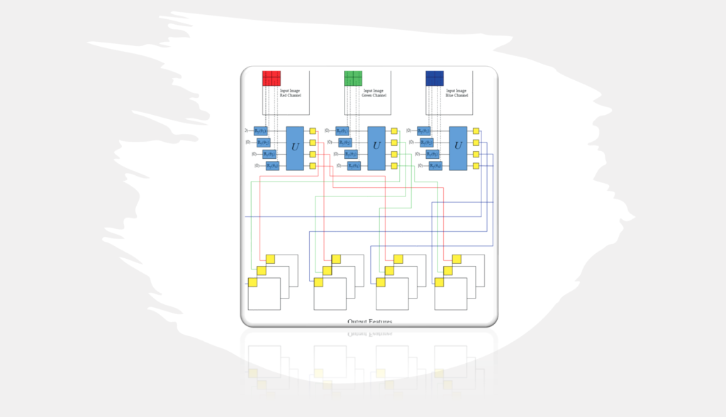
In this demo, I discuss a new type of transformational layer called a quantum convolution, or quanvolutional layer, which locally transforms input data using random quantum circuits, similar to how random convolutional filter layers transform data in convolutional neural networks (CNNs).
A quanvolutional neural network (QCNN) is a type of quantum neural network that uses a quantum circuit to perform convolution operations, which are common in classical convolutional neural networks (CNNs).
In classical CNNs, convolutions are performed using a sliding window technique that extracts local features from the input data. In QCNNs, the convolutional operation is performed using quantum gates, which can be thought of as unitary transformations on quantum states.
The main advantage of QCNNs over classical CNNs is that they can use the inherent parallelism and superposition of quantum computing to perform convolutions more efficiently. This allows for faster and more accurate feature extraction, which is especially useful in image recognition tasks. Quanvolutional neural networks (QNNs) had higher test set accuracy and faster training compared to purely classical CNNs when evaluated on the MNIST dataset. However, QCNNs are still in the early stages of development and are not yet widely used in practice due to the challenges associated with building and training quantum circuits.
QCNNs are still in the early stages of development and are not yet widely used in practice due to the challenges associated with building and training quantum circuits. Here is an implementation of a Quanvolutional image classification using Pennylane and TensorFlow toolkit.

Using a quantum circuit, this code trains a quantum machine learning model to classify handwritten digits from the MNIST dataset. The model uses a convolutional neural network (CNN) architecture, where the same quantum circuit processes each pixel in a 2×2 image. The quantum circuit consists of 4 qubits and is randomly initialized with parameters for each layer. The circuit parameters are optimized using gradient descent over 50 epochs.
The code preprocesses the images by normalizing the pixel values and adding an extra dimension for convolution channels. The quantum pre-processing step is optional, but if enabled, the code applies the quantum circuit to each 2×2 region of the image and saves the results for faster training in future iterations.
The code uses TensorFlow and Keras to build and train the CNN, which has a single dense layer with a softmax activation function for classification. Finally, the code plots the input images and the output channels of the quantum circuit for four samples and saves the model’s training history.
import pennylane as qml
from pennylane import numpy as np
from pennylane.templates import RandomLayers
import tensorflow as tf
from tensorflow import keras
import matplotlib.pyplot as plt


class QuantumImageClassifier:
    def __init__(self, n_epochs=50, n_layers=1, n_train=50, n_test=30,
                 save_path="/", pre_process=True, preprocess_seed=0):
        self.n_epochs = n_epochs
        self.n_layers = n_layers
        self.n_train = n_train
        self.n_test = n_test
        self.save_path = save_path
        self.pre_process = pre_process
        self.preprocess_seed = preprocess_seed

        np.random.seed(preprocess_seed)
        tf.random.set_seed(preprocess_seed)

        self.mnist_dataset = keras.datasets.mnist
        (self.train_images, self.train_labels), (self.test_images, self.test_labels) = self.mnist_dataset.load_data()

        # Reduce dataset size
        self.train_images = self.train_images[:self.n_train]
        self.train_labels = self.train_labels[:self.n_train]
        self.test_images = self.test_images[:self.n_test]
        self.test_labels = self.test_labels[:self.n_test]

        # Normalize pixel values within 0 and 1
        self.train_images = self.train_images / 255
        self.test_images = self.test_images / 255

        # Add extra dimension for convolution channels
        self.train_images = np.array(self.train_images[..., tf.newaxis], requires_grad=False)
        self.test_images = np.array(self.test_images[..., tf.newaxis], requires_grad=False)

        self.dev = qml.device("default.qubit", wires=4)

        # Random circuit parameters
        self.rand_params = np.random.uniform(high=2 * np.pi, size=(self.n_layers, 4))

        @qml.qnode(self.dev)
        def circuit(phi):
            # Encoding of 4 classical input values
            for j in range(4):
                qml.RY(np.pi * phi[j], wires=j)

            # Random quantum circuit
            RandomLayers(self.rand_params, wires=list(range(4)))

            # Measurement producing 4 classical output values
            return [qml.expval(qml.PauliZ(j)) for j in range(4)]

        self.circuit = circuit

    def quanv(self, image):
        """Convolves the input image with many applications of the same quantum circuit."""
        out = np.zeros((14, 14, 4))

        # Loop over the coordinates of the top-left pixel of 2X2 squares
        for j in range(0, 28, 2):
            for k in range(0, 28, 2):
                # Process a squared 2x2 region of the image with a quantum circuit
                q_results = self.circuit(
                    [
                        image[j, k, 0],
                        image[j, k + 1, 0],
                        image[j + 1, k, 0],
                        image[j + 1, k + 1, 0]
                    ]
                )
                # Assign expectation values to different channels of the output pixel (j/2, k/2)
                for c in range(4):
                    out[j // 2, k // 2, c] = q_results[c]
        return out

def preprocess_data(self):
        self.q_train_images = []
        print("Quantum pre-processing of train images:")
        for idx, img in enumerate(self.train_images):
            print("{}/{}        ".format(idx + 1, self.n_train), end="\r")
            self.q_train_images.append(self.quanv(img))
        self.q_train_images = np.asarray(self.q_train_images)

        self.q_test_images = []
        print("\nQuantum pre-processing of test images:")
        for idx, img in enumerate(self.test_images):
            print("{}/{}        ".format(idx + 1, self.n_test), end="\r")
            self.q_test_images.append(self.quanv(img))
            self.q_test_images = np.asarray(self.q_test_images)

        return self.q_train_images, self.q_test_images

def save_preprocess_data(self, q_train_images, q_test_images):

     # Save pre-processed images
    np.save(self.SAVE_PATH + "q_train_images.npy", self.q_train_images)
    np.save(self.SAVE_PATH + "q_test_images.npy", self.q_test_images)

    return True
Here is the line-by-line explanations of each function of the QCNN in detail:
- import pennylane as qml and from pennylane import numpy as np: These lines import the PennyLane library and its accompanying NumPy library for numerical computations.
- from pennylane.templates import RandomLayers: This line imports the RandomLayers function from the PennyLane templates module. The RandomLayers function creates a random quantum circuit of arbitrary depth and connectivity.
- import tensorflow as tf and from tensorflow import keras: These lines import the TensorFlow and Keras libraries, respectively.
- import matplotlib.pyplot as plt: This line imports the Matplotlib library, which is used for data visualization.
- n_epochs = 50: This variable sets the number of optimization epochs for training the model.
- n_layers = 1: This variable sets the number of random layers in the quantum circuit.
- n_train = 50 and n_test = 30: These variables set the number of training and testing samples, respectively.
- SAVE_PATH = “/”: This variable sets the path to the data saving folder.
- PREPROCESS = True: This variable controls whether to perform quantum pre-processing of the input images.
- np.random.seed(0) and tf.random.set_seed(0): These lines set the seeds for the NumPy and TensorFlow random number generators, respectively, to ensure reproducibility of the results.
- mnist_dataset = keras.datasets.mnist: This line loads the MNIST dataset from the Keras library.
- (train_images, train_labels), (test_images, test_labels) = mnist_dataset.load_data(): This line extracts the training and testing images and labels from the MNIST dataset.
- train_images = train_images[:n_train] and train_labels = train_labels[:n_train]: These lines reduce the size of the training dataset to the value of n_train.
- test_images = test_images[:n_test] and test_labels = test_labels[:n_test]: These lines reduce the size of the testing dataset to the value of n_test.
- train_images = train_images / 255 and test_images = test_images / 255: These lines normalize the pixel values of the input images to lie within the range [0, 1].
- train_images = np.array(train_images[…, tf.newaxis], requires_grad=False) and test_images = np.array(test_images[…, tf.newaxis], requires_grad=False): These lines add an extra dimension to the input images to account for convolutional channels.
- dev = qml.device(“default.qubit”, wires=4): This line creates a quantum device on which to execute the quantum circuit. The default.qubit device simulates a quantum computer using classical resources.
- rand_params = np.random.uniform(high=2 * np.pi, size=(n_layers, 4)): This line initializes the random circuit parameters for the quantum circuit. The parameters are drawn uniformly from the range [0, 2π].
- @qml.qnode(dev): This is a Python decorator that creates a quantum node, which is a function that executes a quantum circuit on the specified device.
- def circuit(phi): This is the quantum circuit function that is executed by the quantum node. It takes a list of four classical input values as input and returns a list of four expectation values of the Pauli-Z operator.
- def quanv(image): This function performs the quantum pre-processing of the input image by convolving it with many applications of the same quantum
References:
Henderson, M. (2019). Title of the article. arXiv preprint arXiv:1904.04767, https://doi.org/10.48550/arXiv.1904.04767
